.md .pdf

Contents

Details

Initialization

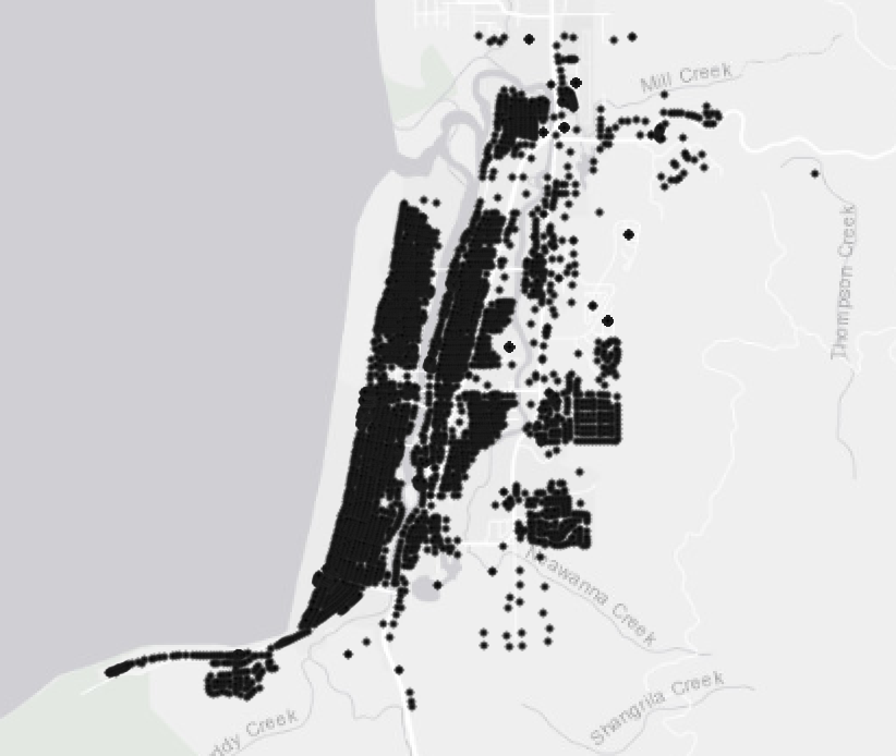
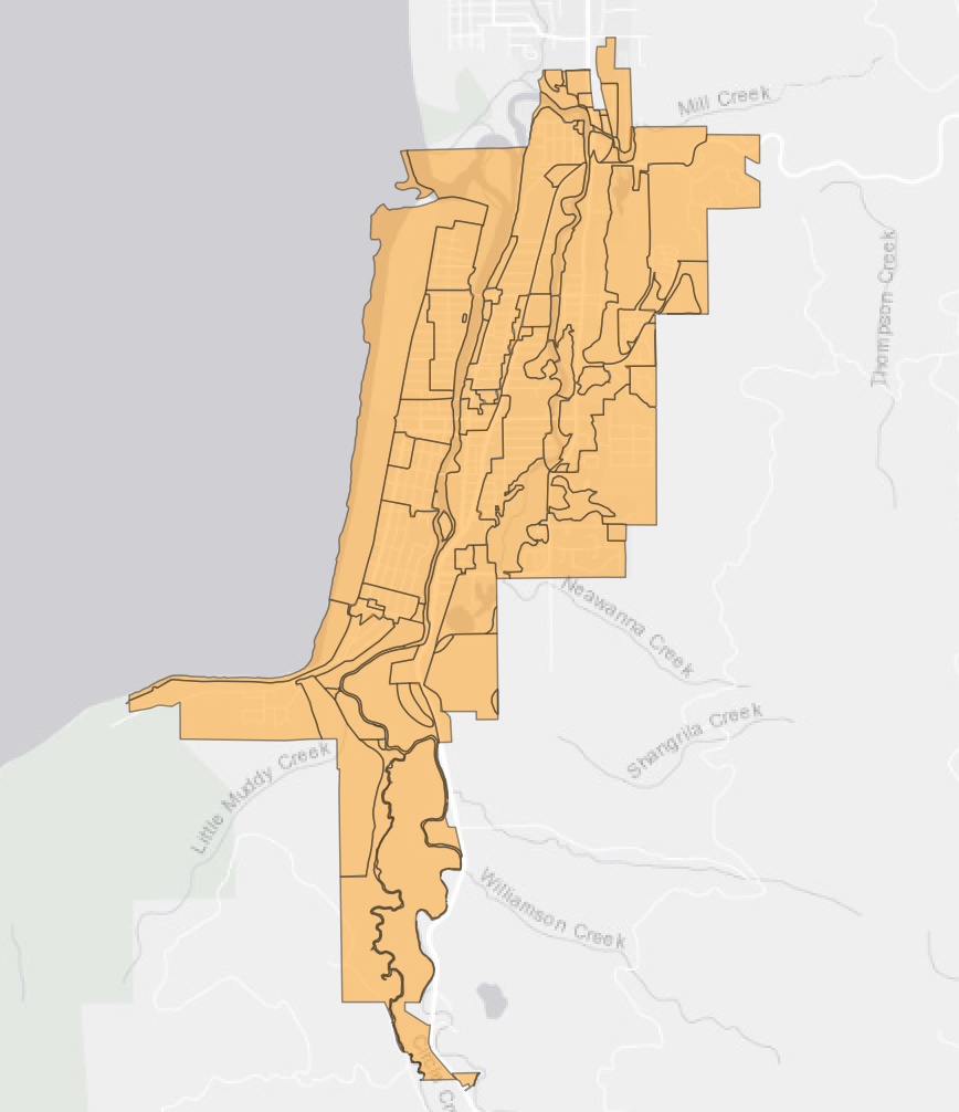
The model is initialized with spatial representations of: (1) parcels in a community, (2) pertinent features such as the coastline, central business district, community assets, and greenspaces, and (3) a zoning layer. With this information, an initial parcel data frame is constructed that represents the parcels and contains spatial information such as the distance to pertinent features and the zone that the parcel is in. A population and housing unit allocation (c in the flowchart representing model processes) stochastically assigns individuals to each parcel using US Census data (Rosenheim et al., 2019). All of the features in this initial data frame are provided in the table below.

Variable	Description
guid	Globally unique identifier for the parcel; if an agent is in a parcel, this is the same as the agent’s “pos”
struct_typ	Structure type; Hazus fragility curves are used for the damage and loss analysis and therefore the structure types are from Hazus; for this work, these include W1 (light-frame wood), W2 (mid-rise wood), C1L (low-rise concrete) and C1M (mid-rise concrete).
year_built	Year of construction or year built
no_stories	Number of stories
dgn_lvl	Design level representing the seismic code the building; units of meters
d_commasst	Distance to community asset; units of meters
d_coast	Distance to coast; units of meters
d_cbd	Distance to central business district; units of meters
zone	Unique identifier for the zone that the parcel is in
zone_type	Type of zone that the parcel is in; options considered here include: open space (OS), residential (R), residential-high density (R_HD), seasonal rental (SR), and commercial (C); additional zones can be considered by modifying the input zoning layer and zoning_params file
numprec	Number of people in the parcel from the housing unit allocation
landuse	Initial land use of the parcel inferred from the housing unit allocation
owner_type	Type of agent that owns the parcel
max_n_agents	Maximum number of agents that can occupy the parcel
x	x-location of the parcel; EPSG:26910 – NAD83/UTM zone 10N is used here
y	y-location of the parcel; EPSG:26910 – NAD83/UTM zone 10N is used here

---

Input

Input to the model consists of both shapefiles and CSZ files.

Shapefiles

The table below describes the shapefiles.

Beach.shp

This is a line layer representing the coast for the model run. An example file is here.

Attribute	Description
ID	ID for beach line

Buildings.shp

This is a point layer representing the buildnigs/parcels for the model run. An example file is here.

Attribute	Description
Guid	Globally unique identifier for the parcel; if an agent is in a parcel, this is the same as the agent’s “pos”
Struct_typ	Structure type; Hazus fragility curves are used for the damage and loss analysis and therefore the structure types are from Hazus; for this work, these include W1 (light-frame wood), W2 (mid-rise wood), C1L (low-rise concrete) and C1M (mid-rise concrete).
Year_built	Year of construction or year built
No_stories	Number of stories
Dgn_lvl	Design level representing the seismic code the building; units of meters

CBD.shp

This is a polygon layer representing the central business district (CBD). An example file is here.

Attribute	Description
ID	ID for central business district

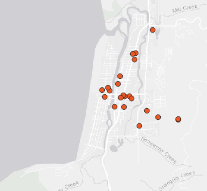
CommunityAssets.shp

This is a point file representing community assets in the model. An example file is here.

Attribute	Description
ID	ID for community assets
Type	Type of community asset (e.g., school, library, hospital)
Name	Name of community asset (e.g., SeasidePostOffice, SeasideFireDepartment)

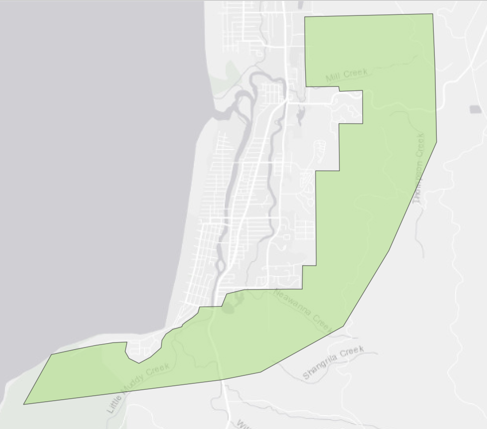
Greenspace.shp

This is a polygon layer representing greenspace in the model. An example file is here.

Attribute	Description
ID	ID for greenspace

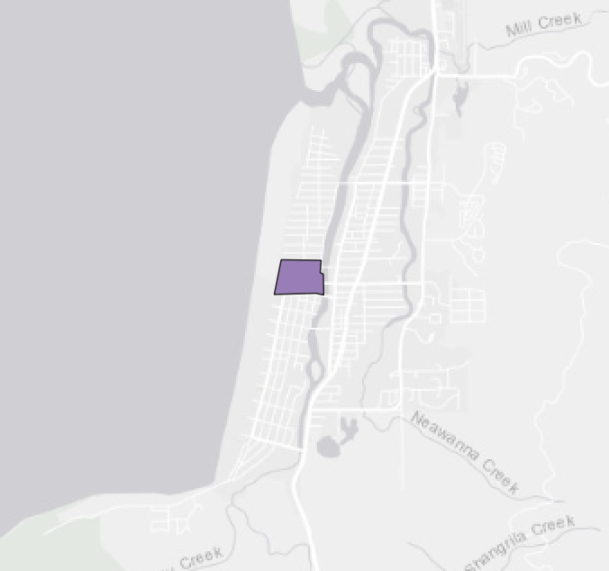
Zoning.shp

This is a polygon layer representing zoning in the model. It needs to align with the zoning.csv file below. An example file is here.

Attribute	Description
guid	Globally unique identifier for zone
zone_abbr	Zone abbreviation; must also be in the zoning_param.csv input file
ZONING	Description of zone

CSV Files

The following CSV files are also read as input to the model.

Input.csv

Provides general input to the model. An example file is here.

Variable	Default Value	Description
n_years	30	number of years to simulate per iteration; time of hazard occurring
n_sims	50	number of simulations/iterations
hazard_recurrence	500	hazard recurrence interval (100, 250, 500, 1000, 2500, 5000, 10000)
seed	1337	seed for simulations
distance_decay_exponent	0.0008	Used to parameterize distance decay function
max_n_LOSR	100000	cap on number of low occupancy seasonal rentals
age_alpha	15	Alpha term for parameterizing gamma distribution for sample of agent age
age_theta	2.667	Theta term for parameterizing gamma distribution for sample of agent age
nhousehold_alpha	5	Alpha term for parameterizing gamma distribution for sample of number of people in household
nhousehold_theta	0.44	Theta term for parameterizing gamma distribution for sample of number of people in household
nvisitor_alpha	10	Alpha term for parameterizing gamma distribution for sample of number of people in visitor group
nvisitor_theta	0.4	Theta term for parameterizing gamma distribution for sample of number of people in visitor group
Household_budget_mean	800	Household agent budget mean; used to parameterize normal distribution
Household_budget_std	200	Household agent budget standard deviation; used to parameterize normal distribution
Household_price_goods	70	Cumulative price of other goods that agent considers when making bid (food, education, entertainment, etc.). Parameterizes WTP
Household_number_parcels_aware	10	number of parcels agent is aware of when searching market
Household_number_searching	400	Constant number of households in model space searching for parcel
Household_change_rate	5	Average number of years that parcel household has same number of people
Landlord_budget_mean	800	Landlord agent budget mean; used to parameterize normal distribution
Landlord_budget_std	200	Landlord agent budget standard deviation; used to parameterize normal distribution
Landlord_price_goods	70	Cumulative price of other goods that agent considers when making bid (food, education, entertainment, etc.). Parameterizes WTP
Landlord_number_parcels_aware	20	number of parcels agent is aware of when searching market
Landlord_number_searching	200	Constant number of landlords in model space searching for parcel
Landlord_transition_penalty	0.35	Penalty for landlord transitioning from one state to another
Firm_budget_mean	2000	Firm agent budget mean; used to parameterize normal distribution
Firm_budget_std	50	Firm agent budget standard deviation; used to parameterize normal distribution
Firm_price_goods	70	Cumulative price of other goods that agent considers when making bid (food, education, entertainment, etc.). Parameterizes WTP
Firm_number_parcels_aware	20	number of parcels agent is aware of when searching market
Firm_number_searching	3	Constant number of firms in model space searching for parcel
Visitor_number_parcels_aware	10	number of parcels agent is aware of when searching market
RealEstate_LandBasePrice	150	Real estate agent base price for land
AllowNew_OwnedRes	1	Boolean for allowing new owned residential development
AllowNew_RentalRes	1	Boolean for allowing new rental residential development
AllowNew_LOSR	1	Boolean for allowing new LOSR development
AllowNew_HOR	1	Boolean for allowing new HOR development
AllowNew_HOSR	1	Boolean for allowing new HOSR development

Zoning_params.csv

Maps the zoning abbreviations to the different land uses. The zoning abbreviations must match those in the Zoning.shp file. Each row corresponds to a zone, and each column to a land use. Default values are provided below. Boolean values are represented as 1 (True) and 0 (False). An example file is here.

Zone	unoccupied	owned_res	rentl_res	ho_res	losr	hosr	comm
OS	1	0	0	0	0	0	0
R	1	1	1	0	1	0	1
R_HD	1	1	1	1	1	0	1
SR	1	0	0	0	1	1	1
C	1	0	0	1	0	1	1

BuildingCodes.csv

Input file describing mandatory building codes when a new change of hands occurs. An example file is here

Variable	Description
from	Initial land use before change of hands
to	New land use that the new owner is considering updating the parcel to
percent_cost	Percent of base price that the building code costs. This is used in the owner WTP calculations.
to_code_level	The code level that the building must go to.
Required	Boolean indicating whether the change is required. Boolean values represented as True/False

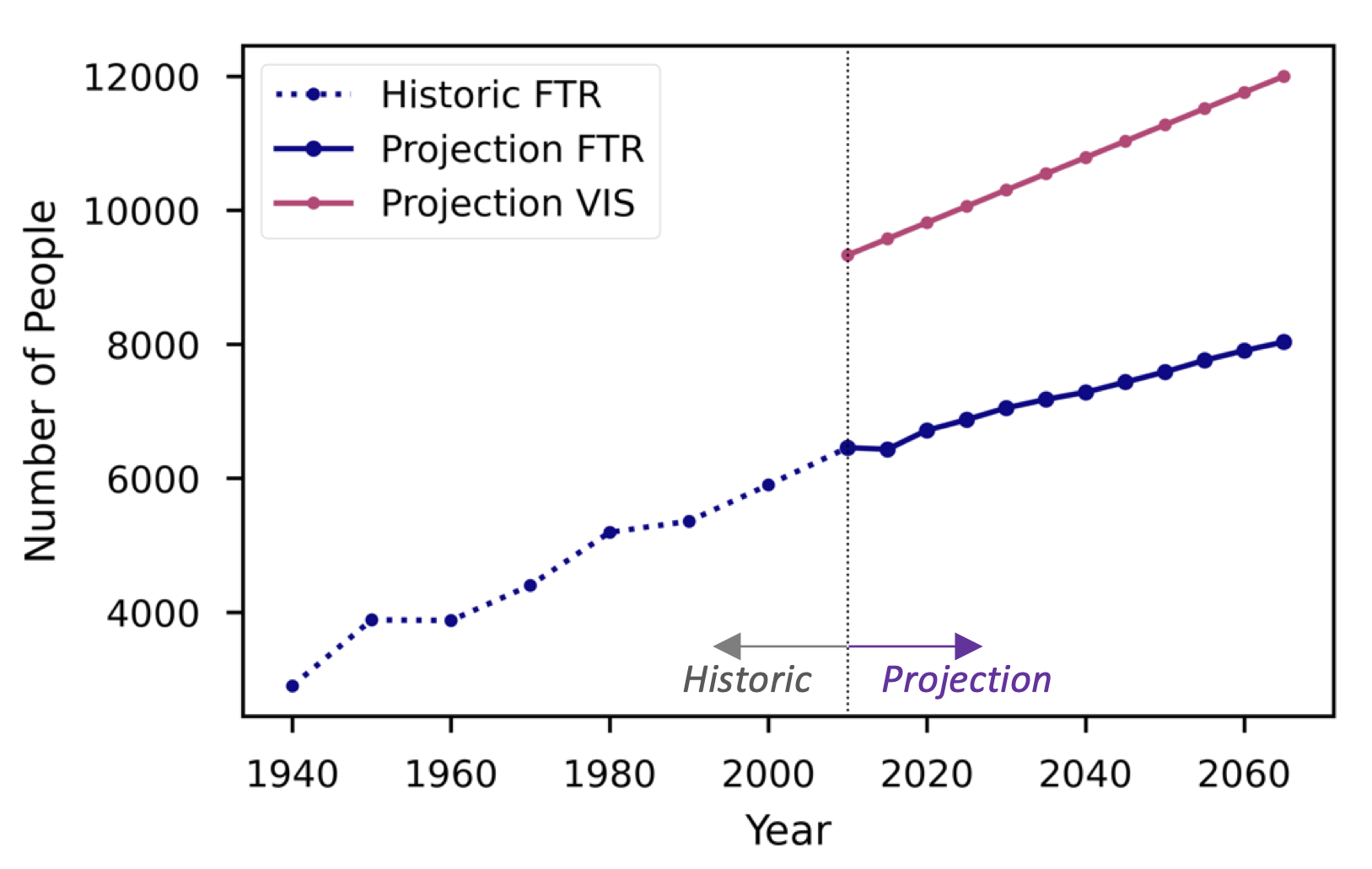
PopulationGrowth.csv

Input file describing deterministic population projections. These are provided for both full time residents and visitors. An example file is here.

Variable	Description
Tick	Time step in model. Starts at 0; must be in 5-year increments
FullTimeResidents	Number of full time at the time step
Visitors	Number of visitors at the time step
Year	Year in actual model; this column is not used in the model, but rather provided for the user

PreferenceMatrix.csv

Matrix describing preferences. If a standard deviation is provided, the preferences are sampled from a normal distribution parameterized on a mean and standard deviation. An example preference matrix is provided below. In this case, a household agent’s preference for parcels near the coast will be sampled from a normal distribution with N(0.3, 0.2). An example file is here.

	household	visitor	Landlord - rentl_res	Landlord - losr	Firm - hor	Firm - hosr
α_coast	0.3	0.7	0.2	0.4	0.15	0.15
α_commast	0.7	-	0.4	-	0.15	-
α_cbd	-	0.3	-	0.2	-	0.15
α_mrkt	-	-	0.4	0.4	0.7	0.7
σ	0.2	0.2	0.1	0.1	0.1	0.1

TaxLot2Bldg.csv

Optional input file that maps tax-lots to a single building. This is provided because some tax-lots in Seaside are contained within a single building (a condo containing multiple tax-lots). In the model, one building is represented as a parcel rather than the many tax-lots located therein. If not using, leave this file blank with the columns provided. An example file is here.

Variable	Description
guid	Globally unique identifier for the parcel
rep_guid	Representative GUID that all parcels in the GUID column will be mapped.
max_n_agents	Maximum number of agents in the building; that is, the number of tax-lots that are represented.

CommercialBuildingMapping.csv

Optional file describing which parcels are commercial buildings in the community. These are assumed static and do not change with this version of the model. If unknown, leave this file blank with the column provided. An example file is here.

Variable	Description
guid	Globally unique identifier of the parcels that are commercial buildings

Submodels

The figure below shows a flowchart representation of the modeling framework. The urban change model is shown with the grey dash-dot box on the left, whereas the hazard consequence model, IN-CORE, is shown with the blue dash-dot box on the right. This section describes each submodel of the flow chart in more detail.

(a) Start

The model starts here Relevant functions:

• main()

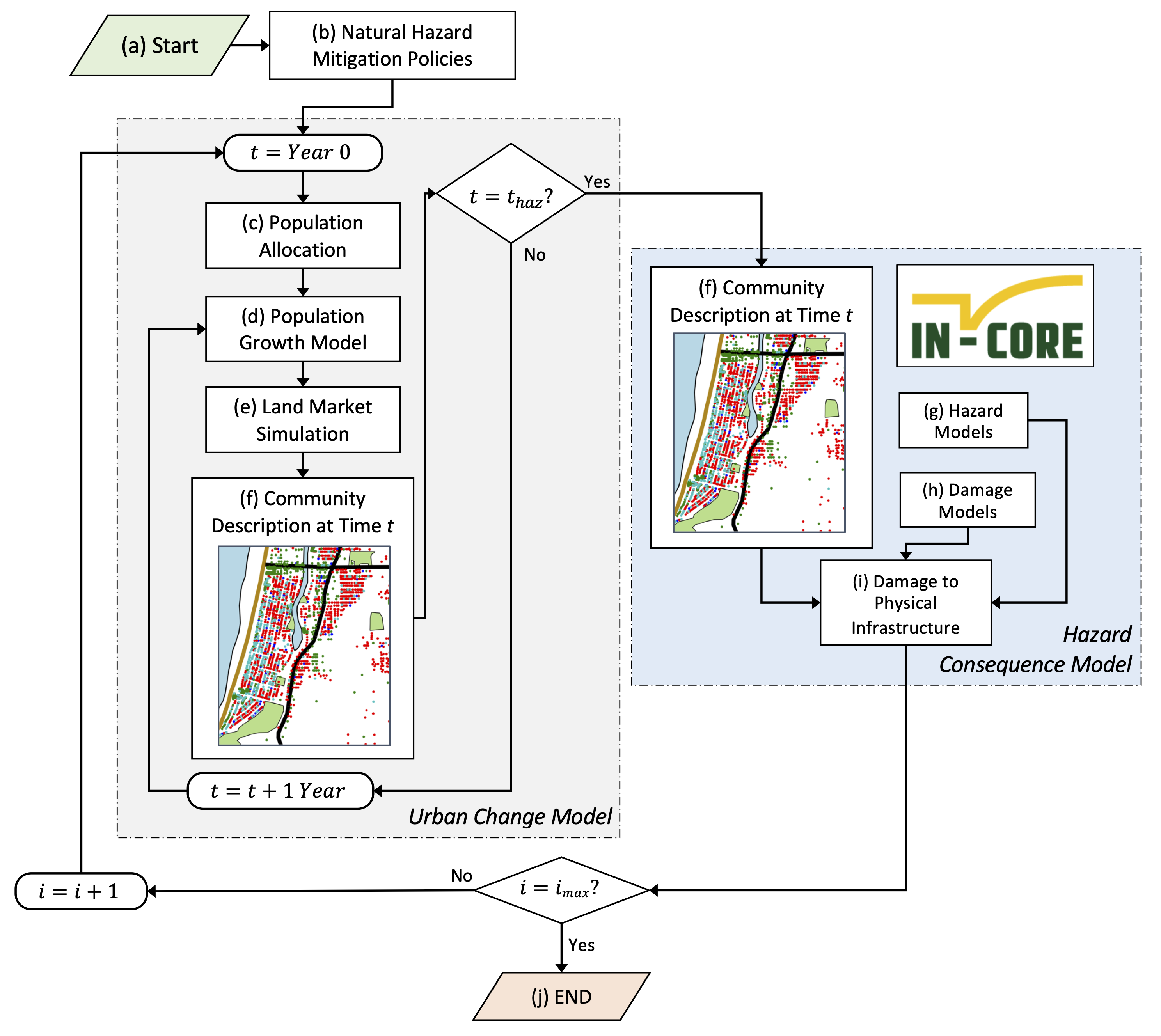
(b) Natural Hazard Mitigation Policies

This is a set of policies that are imposed on the modeling environment and constrains the overall model. By simply modifying the input outlined above, policies to consider could include caps on the number of low occupancy seasonal rental parcels, enforced building codes, relocating community assets, creating new green spaces, rezoning, and limiting new development of particular land uses. The user could also modify the source code to include additional policies outside of those that are controlled by input files.

(c) Population Allocation

This submodel represents the housing unit allocation algorithm in IN-CORE (Rosenheim et al., 2019). This submodel takes publicly available US Census data and stochastically downscales it to the parcel-level. This results in the number of people in each parcel. From the housing unit allocation, the initial land uses are inferred.

Relevant functions:

• housing_unit_allocation()

• assign_property_types()

(d) Population Growth Model

The population growth submodel adds more agents to the model based on the values provided in the input file. Note that this submodel adds agents to the general model space. That is, they are not assigned to a parcel yet, but are in the market looking to purchase a parcel. In this submodel, the household, visitor, landlord, and firm agents are increased. In addition, this submodel represents population outmigration. Population outmigration occurs if the number of people in parcels exceed the values provided in the input file PopulationGrowth.csv.

Relevant functions:

• PopulationGrowth!()

• PopulationOutMigration!()

(e) Land Market Simulation

Household, landlord, and firm agents are competing in a landmarket attempting to purchase parcels that meet their preferences. The landmarket is an extension of the ALMA and ALMA-C models (Filatova et al., 2009; Filatova et al., 2011). The model presented herein considers six agents whereas ALMA only considers two agents: buyer and seller. As in ALMA, agents competing in the land market compute their willingness to pay (WTP) for a parcel. Here, the WTP is modified to account for structural retrofits as:

\[\begin{gather*} WTP = \frac{Y \cdot U^2}{b^2 \cdot U^2}(1+ϵ) - ρ \cdot m \end{gather*}\]

Where Y is the agent budget sampled from a normal distribution, U is the utility of the parcel, b represents costs of other goods, and where ϵ is computed as ϵ=(NB-NS)/(NB+NS), with NB number of buyers and NS number of sellers. The final two terms of the equation above were not in the ALMA model formulation and were added to account for costs associated with structural retrofits. Here, ρ is a constant between 0 and 1 parameterized on the transition between retrofit levels, e.g., low- to moderate-seismic code vs. low- to high-seismic code (see BuildingCodes.csv), and m is the market value of the parcel provided by the real estate agent. This term is subtracted to account for the additional costs an agent would incur if retrofits were mandatory. The utility, U, is computed using a Cobb-Douglas utility function as:

\[\begin{gather*} U = \prod_{i=1}^{n}(P_i^{\alpha_i}) \end{gather*}\]

Where P_i is a normalized value (0-100) representing either proximity to a particular feature or market pressure, α_i weights the importance of this feature to the agent representing preferences, and n are the number of features considered. The preference weights, α, for each agent are sampled from a normal distribution and rescaled such that they sum to 1. Proximity is computed using a scaled distance decay function and market pressure is based on the number of buyers and sellers

\[\begin{gather*} P_{dist} = 100 \cdot e^{-dk} \\ P_{mrkt} = 100 \cdot (0.5\cdot\epsilon + 0.5) \end{gather*}\]

Where d is distance to the feature and k is a tunable parameter.

Relevant functions:

• SimulateVisitorMarketStep!()

• SimulateMarketStep!()

(f) Community Description at Time t

The community description at time t includes the structural properties, seismic codes, land uses, parcel owners, and number of people in each parcel.

Relevant functions:

• UpdateModelCounts!()

(g) Hazard Models

Hazard models are spatially explicit representations of natural hazards. For the Seaside testbed tehse were previously developed as a part of a probabilistic seismic and tsunami hazard analysis (Park et al., 2017; Cox et al., 2022). The PSTHA resulted in hazard maps for seven recurrence intervals (100, 250, 500, 1000, 2500, 5000, and 10000-year). The user can select which hazard recurrence interval to consider as input to the model in Input.csv. The hazard maps are available in the IN-CORE data service which is called at runtime. No hazard layers need to be provided locally.

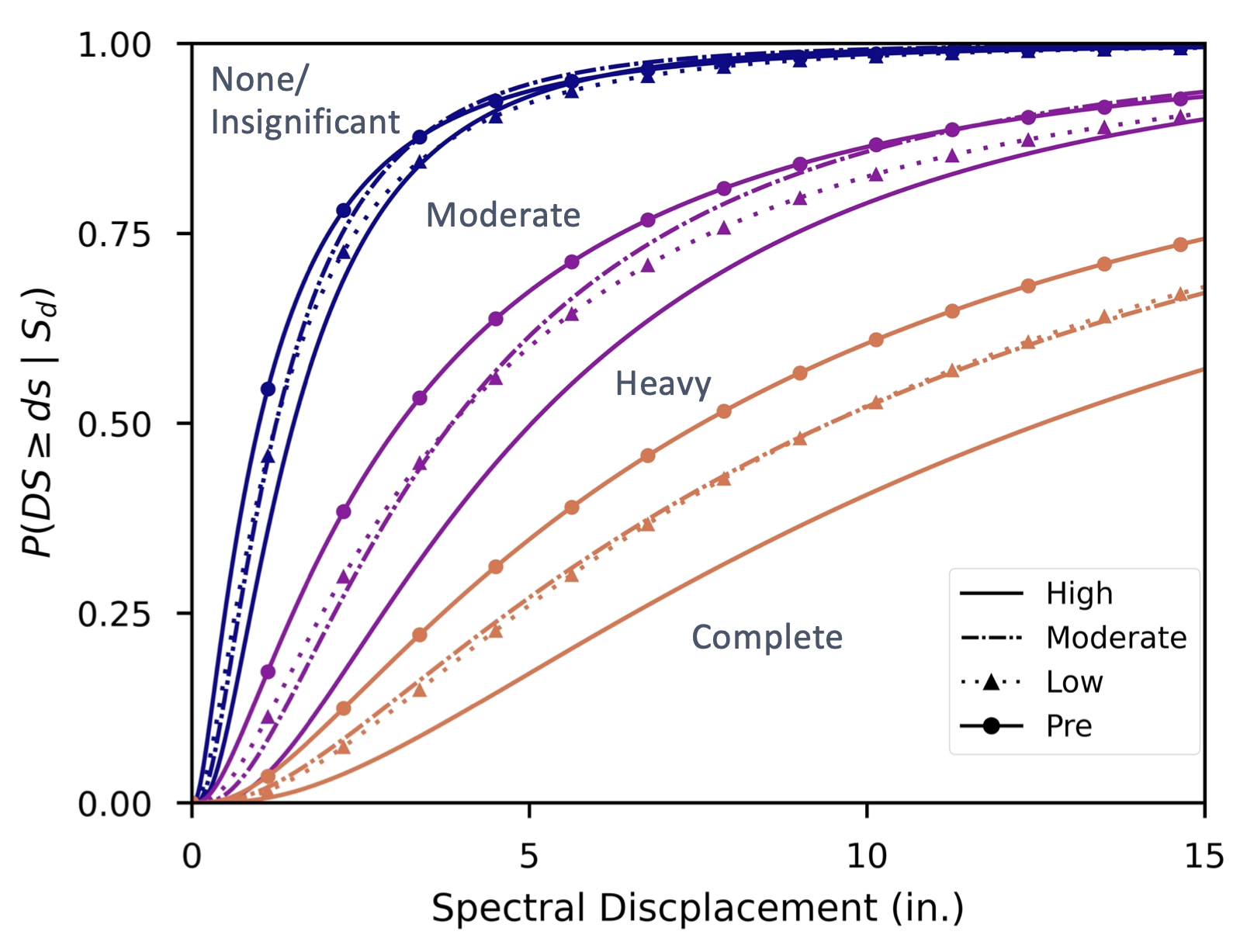
(h) Damage Models

Damage models are fragility functions that describe the probability of exceeding a damage state given a hazard intensity measure. Here Hazus seismic and tsunami fragility curves are employed. The fragility curves are represented as lognormal distribution functions parameterized on a median and dispersion. The fragility curves are mapped to each buildng type and seismic-code level. The fragility curves are available on the IN-CORE data service which is called at runtime and thus not needed locally. The figure below shows an example of seismic fragility curves for a light-frame wood structure for different seismic-code levels.

(i) Damage to Physical Infrastructure

Damage to physical infrastructure is modeled using IN-CORE. IN-CORE maps the spatially explicit hazard intensity measures of (g) to the community description of (f) using the damage models of (h). The hazard occurs in the model at the time step specified by the user in Input.csv. When this step occurs, the model constructs the building data frame necessary to be provided as input to IN-CORE. Using the fragility curves of (h), the probability of each parcel being in different damage states is provided. The expected damage state is computed using these probabilities and one random sample of damage state is computed. Examples of damage to infrastructure include: Park et al., 2019, Kameshwar et al., 2019, and Sanderson et al., 2021.

Relevant functions:

• csz!()

• pyincore_CSZ()

• bldg_dmg_eq()

• bldg_dmg_tsu()

• bldg_dmg_cmltv()

previous

Design Concepts

next

Running the Model